Integrated FLAC3D simulation and field monitoring of bolt-cable supports in three deep coal-mine roadway cases

Appendix A: some theoretical facets of the FLAC^3D software program

FLAC^3D makes use of an express finite-volume formulation to simulate soil, rock, and concrete habits underneath stress and to assemble detailed fashions of tunnels, mines, caverns, and different subsurface buildings. This additionally makes use of an express finite distinction method to suitably discretize the time area right into a sequence of small-time increments. On the graduation of the first-time step, the preliminary stress distribution throughout the mannequin displays the in-situ stress situations; component stresses are assigned in accordance with this preliminary stress area. At this stage, each node displacements and velocities are set to zero, indicating that the mannequin has but to expertise any deformation. Every component retains six parts of the stress tensor. Subsequently, utilizing Cauchy’s components, the distributed forces on the component boundaries might be computed as follows:

the place (:{t}_{i}) denotes the i–th element of the distributed pressure within the i–route, (:{sigma:}_{ij}) represents the interior stress tensor throughout the component, and (:{n}_{j}) stands for the j–th element of the outward unit regular vector to the boundary floor.

Eq. (A1) might be rewritten in a extra expandable method as follows:

Integrating this distributed pressure over the whole boundary yields the full strain on that floor:

the place (:{F}_{i}^{face}) represents the element of the full pressure within the i–route on the boundary floor, (:S) denotes the world of the boundary floor, and (:textual content{d}S) signifies an infinitesimal space of a component on the boundary floor.

Lastly, in accordance with the precept of static equivalence, the full strain is distributed throughout the nodes on the floor. For an everyday boundary floor, the pressure at every node might be acknowledged as:

the place n denotes the variety of nodes on the boundary floor, and (:{F}_{i}^{node}) represents the i–th element of the equal nodal pressure at a single node.

On the whole, the node forces primarily embody the next two varieties:

1. i.

   Gravity pressure

The gravitational pressure ensuing from the self-weight of every component is set by contemplating its quantity, density, and the acceleration attributable to gravity. In accordance with the precept of static equivalence, this gravitational pressure is uniformly allotted among the many nodes of the component:

the place ρ is the component density (kg/m³), V is the component’s quantity (m³), g is the gravitational acceleration (m/s²), n is the variety of nodes per component, and (:{F}_{gravity}) is the equal nodal pressure assigned to a single node (N).

1. ii.

   Stress gradient pressure

The stress is principally concentrated on the middle of every component, representing the stress state of the whole component. When there exists a distinction within the stress on the facilities of adjoining components, the stress gradient might be imagined as follows:

the place (:{sigma:}_{A}:textual content{a}textual content{n}textual content{d}:{sigma:}_{B}) symbolize the stresses on the centroids of two adjoining components, and (:{Delta:}x) denotes the space between the 2 centroids.

This stress gradient causes distributed forces to come up on the frequent interface between adjoining components. Every component calculates the pressure it generates on the frequent interface: the distributed stress (:{sigma:}_{A}^{face}) on the frequent interface of Ingredient A (roughly equal to the centroidal stress (:{sigma:}_{A})) acts uniformly throughout the whole frequent interface, and the full strain might be evaluated by (:{sigma:}_{A}^{face}cdot:{A}_{face}), the place (:{A}_{face}) denotes the world of the frequent interface. This whole strain is distributed to the nodes on the frequent floor in response to the precept of static equivalence, and the equal nodal pressure at every node might be given by (:frac{{sigma:}_{A}^{face}cdot:{A}_{face}}{n}). Equally, the equal nodal pressure distributed to the nodes on the frequent floor for Ingredient B might be calculated as (:frac{{sigma:}_{B}^{face}cdot:{A}_{face}}{n}). On the frequent node, the 2 nodal forces are in reverse instructions, and the unbalanced pressure appearing on the node is expressed by: (:frac{left({sigma:}_{A}^{face}-{sigma:}_{B}^{face}proper)cdot:{A}_{face}}{n}).

1. iii.

   Boundary constraints

The unbalanced pressure (:{overrightarrow{F}}^{unbal}) at a node might be decomposed into three parts: (:{F}_{x}^{unbal},{F}_{y}^{unbal},::textual content{a}textual content{n}textual content{d}:{F}_{z}^{unbal}). When there’s an unbalanced pressure element (:{F}_{ok}^{unbal}) within the ok–route at a node (:left(ok=x,y,zright)), the node tends to displace in that route, and the boundary applies a constraint pressure of (:-{F}_{ok}^{unbal}) to the node in that route.

The mounted assist boundaries prohibit the node’s levels of freedom within the x,y,z–instructions ((:{u}_{x}={u}_{y}={u}_{z}=0)) and applies a constraint pressure (:-{F}_{ok}^{unbal}) in all three instructions to make sure that the node pressure parts in these instructions are zero. The hinged boundaries prohibit solely the node’s displacement freedom within the regular route ((:{u}_{n}=0)) and applies a constraint pressure of (:-{F}_{n}^{unbal}) in that route to make sure the node’s pressure element in that route is zero; there is no such thing as a constraint pressure within the tangential route, so the node can freely slide.

1. iv.

   Analysis of the pretensioning pressure

The prestress is concentrated solely alongside the free size of the rock bolt (anchor cable). Let the endpoints of this free size be represented by factors A and B, the place level A corresponds to the anchor head and level B marks the transition from the free size to the anchored portion. The unit vector directed from node A to node B, aligned with the axis of the bolt, might be expressed as:

the place (:{mathbf{r}}_{A}{:textual content{a}textual content{n}textual content{d}:mathbf{r}}_{B}) denote the place vectors of nodes A and B, respectively, and (:{L}_{f}= parallel {mathbf{r}}_{B}-{mathbf{r}}_{A}parallel) represents the bolt’s free size (m).

The nodal forces appearing on nodes A and B are acknowledged as:

the place for a bolt component with axial stiffness (:{ok}_{b}={E}_{b}{A}_{b}/{L}_{f}), the magnitude of the pretensioning pressure throughout the bolt reads F_pretension =ok_b(u_B–u_A), assuming fixed axial stiffness (no corrosion, no defect, and so forth alongside the bolt’s free size), geometric linearity, solely carrying axial pressure (no bending), displacement compatibility at anchor factors (A and B), and never explicitly modeling the bolt-grout interface shear stress distribution. Within the finite component type, the component pressure can subsequently be thought-about as: (:{mathbf{f}}^{e}={ok}_{b}left[begin{array}{cc}1&:-1:-1&:1end{array}right]{mathbf{u}}^{e}), the place (:{mathbf{u}}^{e}) represents the nodal component displacement.

These node forces type a self-balancing pressure system, satisfying (:{overrightarrow{F}}_{A}+{overrightarrow{F}}_{B}=0). Assuming that the bolt doesn’t endure rigid-body translational or rotational movement and no exterior forces are exerted on the free size. It must be famous that if the bolt is totally grouted alongside its complete size (not simply anchored on the ends), the formulation ought to embody steady shear stress switch alongside the bolt-grout interface, usually utilizing a spring-slider mannequin (e.g., Itasca FLAC/UDEC cable components). The simplified two-node truss mannequin is suitable for end-anchored bolts however not for totally grouted bolts.

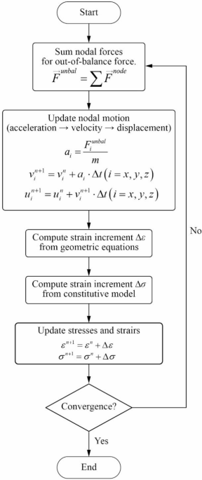
Taking the vector sum of all node forces yields the unbalanced pressure on the node (:{overrightarrow{F}}^{unbal}=sum:{overrightarrow{F}}^{node}). In accordance with Newton’s second regulation, the acceleration vector of the node takes the next type: (:{a}_{i}=frac{{F}_{i}^{unbal}}{m}), the place m represents the mass of the node. That is employed to replace the rate vector of the node (:{v}_{i}^{n+1}={v}_{i}^{n}+{a}_{i}{Delta:}t), and subsequently replace the displacement vector (:{u}_{i}^{n+1}={u}_{i}^{n}+{v}_{i}^{n+1}cdot:{Delta:}tleft(i=x,y,zright)).

The variations in node displacement trigger component deformation. At every time step, the node displacement increment might be thought-about as (:{Delta:}{u}_{i}={u}_{i}^{n+1}-{u}_{i}^{n}={u}_{i}^{n}+{v}_{i}^{n+1}{Delta:}t-{u}_{i}^{n}={v}_{i}^{n+1}cdot:{Delta:}tleft(i=x,y,zright)). Utilizing the incremental type of the geometric equations, the pressure increment (:{Delta:}{epsilon:}_{ij}) for the present time step within the context of small deformation (i.e., small strains) might be readily expressed by:

the place (:{Delta:}{u}_{i}:textual content{a}textual content{n}textual content{d}:{Delta:}{u}_{j}) symbolize the parts of the displacement increment within the i and j instructions, respectively; x_i and x_j are the spatial coordinate parts such that (:{x}_{x}=x,:{x}_{y}=y,{:textual content{a}textual content{n}textual content{d}:x}_{z}=z).

Within the case of (:i=j), the parts of the conventional pressure increment are readily derived as:

whereas within the case of (:ine:j), the parts of the shear pressure increment take the next type:

By including the incremental pressure tensor to the component’s pressure tensor, one can arrive on the following recursion relation:

the place (:{epsilon:}_{ij}^{n}:textual content{a}textual content{n}textual content{d}:{epsilon:}_{ij}^{n+1}) so as are the pressure tensors of the component on the finish of the earlier time step and the present time step, and (:{Delta:}{epsilon:}_{ij}) represents the pressure increment of the present time step. It’s also value mentioning that the appliance restrict of Eqs. (A11a) and (A11b) are small-strain issues, incremental linearity, no rigid-body contamination, and goal stress charge. For giant-strain issues, frequent in underground excavations with yielding rock, Inexperienced–Lagrange pressure and goal stress charges are required and these must be appropriately integrated into the incremental strains.

Primarily based on the fabric’s constitutive relationship, the corresponding stress increment (:{Delta:}{sigma:}_{ij}) might be evaluated by way of the pressure increment (:{Delta:}{epsilon:}_{ij}). The 2 constitutive fashions used on this paper are as follows:

1. 1.

   Mohr–Coulomb constitutive mannequin

The Mohr–Coulomb mannequin is principally relevant to rock formations reminiscent of sandstone and shale, and its yield criterion is acknowledged as:

On the whole, the principal stress represents a three-dimensional house outlined by the three principal stresses (:{sigma:}_{1},{sigma:}_{2},{textual content{a}textual content{n}textual content{d}:sigma:}_{3}) as coordinate axes, with (:{sigma:}_{1}ge:{sigma:}_{2}ge:{:sigma:}_{3}) (compression unfavourable in FLAC^3D) and every level (:left({sigma:}_{1},{sigma:}_{2},{sigma:}_{3}proper)) within the house corresponds to a stress state. The yield floor is characterised because the boundary separating the elastic area from the plastic area on this house. Within the case of (:{f}_{s}left({sigma:}_{ij}proper)<0), the stress level mendacity contained in the yield floor, and the fabric stays within the elastic state; whereas for the case of (:{f}_{s}left({sigma:}_{ij}proper)=0), the stress level lies on the yield floor, and the fabric enters the plastic state. As well as, there aren’t any corresponding true stress factors within the area for the case of (:{f}_{s}left({sigma:}_{ij}proper)>0).

In FLAC^3D, the steps used for calculating take a look at stresses are as follows:

Assuming the fabric is within the elastic state, the elastic stress increment ((:{Delta:}{sigma:}_{ij}^{e})) might be calculated in response to the next elastic constitutive relationship:

the place (:{D}_{ijkl}^{e}) denotes the fourth-order elastic constitutive tensor (MPa). For homogeneous-elastic-isotropic supplies, Eq. (A14) might be acknowledged in a extra expandable method:

the place (:E) denotes the elastic modulus of the fabric (MPa), and (:nu:) represents the Poisson’s ratio of the fabric.

By including the elastic stress increment ((:varDelta:{sigma:}_{ij}^{e})) to the stress ((:{sigma:}_{ij}^{n})) from the earlier time step, one can get hold of the take a look at stress ((:{sigma:}_{ij}^{trial})) for the present time step as follows:

If (:{f}_{s}left({sigma:}_{ij}^{trial}proper)<0), the stress on the present time step is offered by (:{sigma:}_{ij}^{n+1}={sigma:}_{ij}^{trial}); and if (:{f}_{s}left({sigma:}_{ij}^{trial}proper)ge:0), the radial regression algorithm is utilized to map the take a look at stress factors onto the yield floor alongside the conventional route (for coupled stream) or the route of the plastic potential gradient (for uncoupled stream), and the corresponding plastic pressure increment (:{Delta:}{epsilon:}_{ij}^{p}) is then evaluated.

Within the case of (:{f}_{s}left({sigma:}_{ij}^{trial}proper)ge:0), based mostly on the small-deformation assumption, the pressure increment on the present time step might be rationally predicted by linearly superimposing the elastic pressure increment and the plastic pressure increment within the following type:

In accordance with the elastic constitutive relationship, the elastic stress increment might be linearly associated to the elastic pressure increment within the following type (:varDelta:{sigma:}_{ij}={D}_{ijkl}^{e}varDelta:{epsilon:}_{kl}^{e}). The stress correction attributable to plastic deformation for the present time step might be modified by:

the place (:-{D}_{ijkl}^{e}:{Delta:}{epsilon:}_{kl}^{p}) denotes the plastic stress correction time period.

The route of the gradient of the plastic potential operate is coincident with the route of plastic stream, such that the incremental plastic pressure ((:{Delta:}{epsilon:}_{ij}^{p})) happens on this route and might be acknowledged by:

the place (:varDelta:lambda:) represents the plastic multiplier, (:{overrightarrow{n}}_{ij}) is the unit tensor within the plastic stream route, (:gleft({sigma:}_{ij}proper)) signifies the plastic potential operate, and (:frac{partial:gleft({sigma:}_{ij}proper)}{partial:{sigma:}_{ij}}) denotes the gradient of the plastic potential.

By incorporating the unit tensor into the plasticity matrix, the expression might be simplified to:

The incremental plastic pressure ((:{Delta:}{epsilon:}_{ij}^{p})) represents a diagonal tensor; in view of (:frac{partial:gleft({sigma:}_{ij}proper)}{partial:{sigma:}_{2}}=0) (i.e., (:varDelta:{epsilon:}_{2}^{p}=0)), its particular configuration takes the next type:

Now, by substituting Eq. (A20a) into Eq. (A18), it’s obtainable:

For the Mohr–Coulomb constitutive mannequin, a non-associated stream rule is adopted, and the route of the plastic pressure increment follows the gradient of the plastic potential. By this advantage, the plastic potential operate (:gleft({sigma:}_{ij}proper)) might be acknowledged as:

the place (:psi:) denotes the dilation angle of the fabric.

Typically, the case of (:psi:le:varphi:) represents the non-associated stream; if ψ = 0, the plastic quantity change can be zero throughout shear (incompressible plastic stream). Within the case of (:psi:=varphi:), the plastic potential operate (:gleft({sigma:}_{ij}proper)) takes the identical type because the yield operate (:{f}_{s}left({sigma:}_{ij}proper)), and the non-conformal stream rule degenerates into the conformal stream rule.

Via evaluating the first-order partial derivatives of the plastic potential operate (:gleft({sigma:}_{ij}proper)), the plastic potential gradient is obtained as follows:

Within the principal stress house, the yield floor of the Mohr–Coulomb constitutive mannequin represents a hexagonal pyramid, and the by-product of the yield operate (:{f}_{s}left({sigma:}_{ij}proper)) doesn’t exist on the edges and vertices; nonetheless, for a take a look at stress level (:{sigma:}_{ij}^{trial}) removed from the perimeters and vertices, the yield operate is differentiable. Due to this fact, its first-order Taylor growth close to (:{sigma:}_{ij}^{trial}) might be expressed as:

By truncating the higher-order phrases of the Taylor sequence, the first-order linear approximation might be derived within the following type:

By introducing Eq. (27) into Eq. (31),

After rearrangement, it may be readily acknowledged as:

From the consistency situation (:{f}_{s}left({sigma:}_{ij}^{n+1}proper)=0), the plastic multiplier ((:{Delta:}lambda:)) might be evaluated as:

The primary-order partial derivatives of the yield operate (:{f}_{s}left({sigma:}_{ij}proper)) and the plasticity potential operate (:gleft({sigma:}_{kl}proper)) with respect to the principal stress are:

By substituting Eqs. (A29a) and (A29b) into Eq. (A28), one can arrive at:

As well as, via substituting Eq. (A30) again into Eq. (A22), the corrected stress (:{sigma:}_{ij}^{new}) on the present time step might be derived as:

1. 2.

   Pressure-softening constitutive mannequin

The coal seam is modeled utilizing a strain-softening constitutive mannequin, whose yield criterion is equivalent to that of the Mohr–Coulomb mannequin; nonetheless, the interior friction angle (φ) and the cohesion (c) are monotonically lowering features of the softening parameter ((:kappa:)), i.e.:

the place (:kappa:=sqrt{frac{2}{3}{e}_{ij}^{p}{e}_{ij}^{p}}) (:kappa:=int:sqrt{frac{2}{3}{dot{e}}_{ij}^{p}{dot{e}}_{ij}^{p}}textual content{d}t), through which e_ij denotes the deviatoric a part of (:{epsilon}_{ij}). Typically, the trial stress on the present time step is given by (:{sigma:}_{ij}^{trial}={sigma:}_{ij}^{n}+{D}_{ijkl}^{e}{Delta:}{epsilon:}_{kl}). If (:{f}_{s}left({sigma:}_{ij}^{trial},{kappa:}^{n}proper)<0), then the stress on the present time step takes the next type: (:{sigma:}_{ij}^{n+1}={sigma:}_{ij}^{trial}); if (:{f}_{s}left({sigma:}_{ij}^{trial},{kappa:}^{n}proper)ge:0), the radial regression algorithm is adopted to map the take a look at stress level to the yield floor alongside the route of the plastic potential gradient.

The plastic pressure increment ((:{Delta:}{epsilon:}_{ij}^{p})) on the present time step is given by:

Via updating the softening parameter ((:kappa:)) based mostly on (:{Delta:}{epsilon:}_{ij}^{p}), one can arrive at:

Then, the softening parameter (:{kappa:}^{n+1}) for the present time step takes the next type:

By updating the interior friction angle ((:varphi:)) and cohesion ((:c)) of the coal physique based mostly on (:{kappa:}^{n+1}), one can arrive at:

the place (:{varphi:}_{0}:textual content{a}textual content{n}textual content{d}:{varphi:}_{r}) so as are the preliminary and residual friction angles of the coal mass (°), (:{c}_{o}::textual content{a}textual content{n}textual content{d}:{c}_{r}) are the preliminary and residual cohesions of the coal mass (MPa), whereas (:{kappa:}_{1}::textual content{a}textual content{n}textual content{d}:{kappa:}_{2}) are the pressure thresholds for the onset and termination of pressure softening, respectively.

The present time-step-corrected stress ((:{sigma:}_{ij}^{n+1})) is calculated by:

Now, allow us to add the stress increment tensor to the component’s stress tensor:

the place (:{sigma:}_{ij}^{n}:textual content{a}textual content{n}textual content{d}:{sigma:}_{ij}^{n+1}) are the stress tensors of the component on the finish of the earlier time step and the present time step, respectively, and (:{Delta:}{sigma:}_{ij}) represents the stress increment of the present time step.

The up to date stresses on the present time step are utilized because the preliminary stresses for the following time step; the nodal forces are then recalculated, and the iteration proceeds to the next time step. Because the variety of iterations will increase, the unbalanced forces on the nodes progressively converge, in the end main the mannequin to attain static equilibrium. For this, the convergence standards are taken as follows:

the place (:{F}_{kx},{F}_{ky},{textual content{a}textual content{n}textual content{d}:F}_{kz}) symbolize the parts of the nodal pressure within the x, y,z–instructions on the ok–th node, respectively, N denotes the full variety of nodes within the mannequin; (:{overrightarrow{F}}_{ok}) is the nodal pressure vector on the ok–th node; (:{overline{F}}_{node}) is the typical magnitude of all nodal forces; and (:{F}_{max}^{unbal}) is the utmost magnitude of the resultant nodal pressure vector.

The computational process of the specific answer scheme for every time step in FLAC^3D is offered in Determine A1.

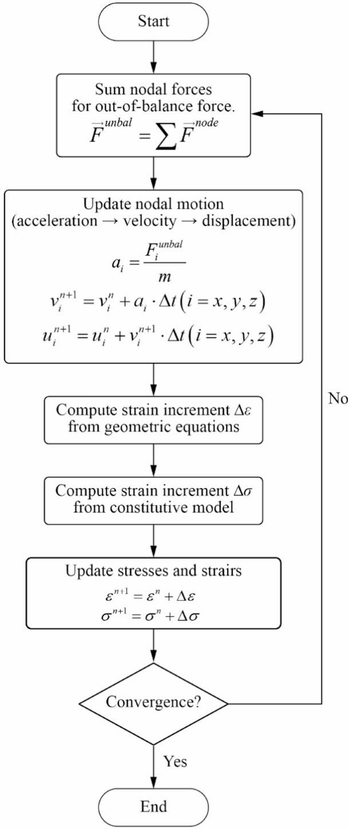
Computational flowchart of the specific answer scheme for a single timestep in FLAC^3D.