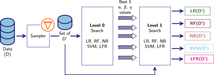

Overview of the proposed strategy.
Within the exploratory evaluation, we noticed that the best way we construction the stability within the coaching dataset impacts the classification equity and accuracy. Then, the subsequent step is looking for an optimum stability construction for the dataset that may present the absolute best classification equity and accuracy. To this goal, we mannequin this drawback as a multi-criteria optimization drawback and suggest a search-based resolution searching for the optimum stability for beneficial vs. unfavourable labels and privileged vs. unprivileged teams within the information.
Subsequently, the proposed resolution is model-agnostic, and it may be used along with any classification algorithm, in addition to with different debiasing strategies.
The proposed methodology has two fundamental elements:
-
Sampling in accordance with a given stability construction, and
-
Grid search to search out the optimum stability construction.
The overview of the proposed resolution is given in Fig. 1. In the remainder of this part, these elements are described in additional element.
Sampling in accordance with a given stability construction
Within the proposed methodology, given the unique information assortment D, the objective is to assemble a sampled dataset (D’) which has a sure goal stability construction. The sampled assortment (D’) consists of the next 4 partitions:
-
(p_{f}’) : privileged beneficial samples
-
(p_{uf}’) : privileged unfavourable samples
-
(up_{f}’) : unprivileged beneficial samples
-
(up_{uf}’) : unprivileged unfavorable samples
On this notation, (p’) denotes the set of all privileged customers, each with favorable and unfavorable labels, and (up’) denotes the set of all unprivileged customers. Equally, (f’) denotes the set of all favorably labeled customers, each in privileged and unprivileged teams, and (uf’) denotes the set of all unfavorably labeled customers. The counterparts of those variables with out ’ denote the corresponding units in D.
There are fundamental ideas to think about when sampling from the unique information. Machine studying strategies which can be historically developed to maximise accuracy, usually skew their predictions in the direction of the bulk class. We hypothesize that (D’) samplings which can be of upper imbalance than D, is not going to profit our optimization efforts. Thus, we are not looking for the make the imbalance in both of the favourability and privilege axes to be increased in our sampling (D’) than that of the unique information D. One other restriction we wish to incorporate in our methodology is that we are not looking for the bulk class in D to be the minority within the D’ in both of the favourability and privilege axes. Moreover, the speed of the beneficial labels within the privileged and unprivileged teams shouldn’t be modified such that the speed of beneficial situations within the unprivileged group exceeds the speed throughout the privileged group. In different phrases, the privileged/unprivileged teams shouldn’t interchange the roles when it comes to bias. These restrictions are listed as follows:
-
1.
The bulk privilege group’s ratio in (D’) can’t be increased than that of D.
-
2.
The bulk privilege group in D can’t be the minority group in (D’)
-
3.
The bulk favourability label’s ratio in (D’) can’t be increased than D. This additionally signifies that the minority favourability label’s ratio can’t be lower than in D.
-
4.
The bulk favourability group in D can’t be the minority group in (D’)
-
5.
The privileged group’s benefit over the unprivileged group in getting beneficial label shall not be extra in (D’) than D.
-
6.
The unprivileged group can’t be extra prone to be assigned to the beneficial label than the priviledged group, in different phrases, the privileged/unprivileged teams shouldn’t interchange the roles when it comes to bias.
The formal descriptions of those restrictions are as given in Equation 3.
$$start{aligned} start{aligned} textual content {Restrictions 1 and a couple of: }&fracD’ in R(fracpD,0.5) textual content {Restrictions 3 and 4: }&fracD’ in R(fracfD,0.5) textual content {Restrictions 5 and 6: }&frac{frac{|p_{f}’|}}{frac{|up_{f}’|}} in R(frac{frac{|p_{f}|}p}{frac{|up_{f}|}},1) finish{aligned} finish{aligned}$$
(3)
Right here, R(x, y) is the closed interval between x and y, as given in Equation 4.
$$start{aligned} start{aligned} R(x,y)= {left{ start{array}{ll} {}[x,y] & xle y {}[y,x] & in any other case finish{array}proper. } finish{aligned} finish{aligned}$$
(4)
The sampling to assemble (D’) below the above restrictions, fulfilling a desired stability construction (stability ratio), is carried out utilizing the next three parameters, every having values in [0,1]:
-
Parameter (alpha): It controls the unprivileged group fee inside (D’). When it’s set to 0, (D’) has the identical fee of unprivileged group situations as in D. The worth 1 constrains the unprivileged group fee to be 0.5, i.e. half of the situations within the delicate attribute. For any worth in (0,1) this fee might be computed from the linear interpolation of those two finish factors.
-
Parameter (beta): It controls the unfavourable labeled occasion fee inside (D’). When it’s set to 0, (D’) has the identical fee of unfavourable labels as in D, whereas the worth 1 makes this fee equal to 0.5. As in (alpha), for any worth in (0,1) this fee might be computed from the linear interpolation of those two finish factors.
-
Parameter (gamma): It controls the ratio of the privileged group in comparison with the unprivileged group in getting assigned the beneficial label. With the worth 0, (D’) has the identical ratio as in D, whereas the worth 1 makes the ratio equal to 1, giving equal favourability charges to the privileged and unprivileged teams. As within the different two parameters, for any worth in [0,1], this fee might be computed from the linear interpolation of those two endpoints.
Given these three parameters, the scale of the partitions for (p_f’), (p_uf’), (up_f’) and (up_uf’) might be unambiguously decided. The partition ratios are numerically obtained from the constraints in Equation 5.
$$start{aligned} start{aligned} textual content {1. }&fracD’ = fracpD(1-alpha )+0.5*alpha textual content {2. }&fracD’ = fracfD(1-beta )+0.5*beta textual content {3. }&frac{frac{|p_{f}’|}}{frac{|up_{f}’|}} = frac{frac{|p_{f}|}p}{frac{|up_{f}|}}*(1-gamma )+gamma finish{aligned} finish{aligned}$$
(5)
This formulation has the benefit of being interpretable such that (alpha) might be interpreted because the balancing quantity within the privileged/unprivileged axis, (beta) because the balancing quantity within the beneficial/unfavourable axis, and (gamma) is interpretable as an element that governs the stability of the favourability charges of the completely different privilege lessons.
In an effort to stop dataset dimension to be an element affecting the sampling outcomes, as soon as the computation of the sampling ratios for every ((alpha ,beta ,gamma )in {0,0.01,0.02,…,1}^3) is accomplished, we discover the utmost dimension of (D’), such that for every (alpha , beta , gamma) mixture the computed sampling ratios are satisfiable given the occasion counts ((p_{f}), (p_{uf}), (up_{f}),(up_{uf})) in D.
The calculation of the sampling ratios ((frac{|p_{f}’|}D’), (frac{|p_{uf}’|}D’), (frac{|up_{f}’|}D’),(frac{|up_{uf}’|}D’)) from the aforementioned constraints is given in Equation 6.
$$start{aligned} start{aligned} P’ =&fracD’ = fracpD(1-alpha )+0.5*alpha F’ =&fracD’ = fracfD(1-beta )+0.5*beta A’ =&frac{frac{|p_{f}’|}}{frac{|up_{f}’|}} = frac{frac{|p_{f}|}p}{frac{|up_{f}|}}*(1-gamma )+gamma finish{aligned} finish{aligned}$$
(6)
On condition that (F_{p}’=frac{|p_{f}’|}) and (F_{up}’=frac{|up_{f}’|}), Equation 7 exhibits methods to compute (F_{up}’).
$$start{aligned} start{aligned} F_{p}’&= A’*F_{up}’ F’&= P’*F_p’+(1-P’)*F_{up}’&=P’*(A’*F_{up}’)+(1-P’)*F_{up}’ &= F_{up}’*(1+A’P’-P’), then F_{up}’&= frac{F’}{(1+A’P’-P’)} finish{aligned} finish{aligned}$$
(7)
As soon as (F_{up}’) is computed, (F_{p}’=frac{|p_{f}’|}) might be trivially computed as (F_{up}’ * A’). Then the equations for the computing the sampling ratios are as given in Equation 8.
$$start{aligned} start{aligned} frac{|p_{f}’|}D’&= P’*F_p’ frac{|p_{uf}’|}D’&= P’*(1-F_p’) frac{|up_{f}’|}D’&= (1-P’)*F_{up}’ frac{|up_{uf}’|}D’&= (1-P’)*(1-F_{up}’) finish{aligned} finish{aligned}$$
(8)
Instance. Given a dataset D and parameters (alpha ,beta ,gamma), we display how the scale of the partitions is decided from Equation 8 to acquire the pattern. Suppose that the preliminary dataset D has the distribution as given in Desk 5. For the parameters (alpha =0.5,beta =0.8,gamma =0.4), by utilizing Equation 8, we compute the sampling ratios and the corresponding higher bounds on (|D’|) as follows:
-
(frac{|p_{f}’|}D’ approx 0.421 Longrightarrow |D’| le fracp_f{frac{|p_{f}’|}D’} approx frac{19500}{0.421} = 46318)
-
(frac{|p_{uf}’|}D’ approx 0.284 Longrightarrow |D’| le frac{frac{|p_{uf}’|}D’} approx frac{500}{0.28} = 1761)
-
(frac{|up_{f}’|}D’ approx 0.176 Longrightarrow |D’| le frac{frac{|up_{f}’|}D’} approx frac{1900}{0.176} = 10795)
-
(frac{|up_{uf}’|}D’ approx 0.120 Longrightarrow |D’| le frac{frac{|up_{uf}’|}D’} approx frac{100}{0.120} = 833)
Though computing the ratios on ((alpha ,beta ,theta )=(0.5,0.8,0.4)) yields the tightest higher sure on (|D’|) as 909, computing on all ((alpha ,beta ,theta )in {0,0.01,0.02,,1}^3) would possibly yield a a lot tighter higher sure. Certainly performing the iteration on ((alpha ,beta ,theta )in {0,0.01,0.02,,1}^3) yields a decrease higher sure of (|D’| le 394). Utilizing this decrease sure, the pattern composition is as given in Desk 6.
Grid search to search out the optimum stability construction
On condition that the stability construction within the pattern is expressed utilizing the parameters (alpha , beta) and (gamma), grid search is used for locating the parameter values that produce the optimum outcomes with respect to equity and classification accuracy.
Because the drawback incurs two metrics to optimise, (DI_RATIO) for equity and MCC metrics for classification accuracy by, the answer is obtained by multi-criteria optimisation strategy. The loss features associated to (DI_RATIO) and MCC as given in Equation 9 and Equation 10, respectively.
$$start{aligned} DI_RATIO_LOSS = |1-DI_RATIO| finish{aligned}$$
(9)
$$start{aligned} MCC_LOSS = |1-MCC| finish{aligned}$$
(10)
A mixed loss perform is outlined as in Equation 11.
$$start{aligned} COMBINED_LOSS = c_1*MCC_LOSS + c_2* DI_RATIO_LOSS finish{aligned}$$
(11)
Because the proposed strategy is model-agnostic, the sampling strategy might be utilized earlier than any equity methodology, and it may be used for setting up the coaching dataset of any classification mannequin. The (DI_RATIO) and MCC values can then be obtained for any given classifier. On this examine, LR, RF, SVM, and NB classifiers are used. Given the dataset D and the stability construction parameters ((alpha , beta) and (gamma)), we are able to examine the efficiency of a given classification mannequin by Algorithm 1.
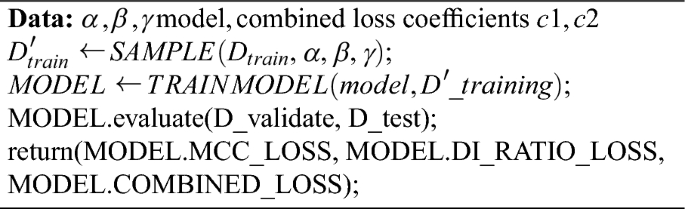
On this algorithm, initially, a pattern (D’_{practice}) is constructed. Then the classification mannequin is educated by utilizing (D’_{practice}), after which it’s evaluated on the validation and take a look at partitions of D. This analysis returns the loss values in addition to the mixed loss worth of the mannequin. To accommodate two stage search and stop information leakage, two completely different (D_{take a look at}) units are constructed in the beginning and every stage makes use of its personal take a look at set.
Grid Search Grid search is usually used for hyper-parameter optimization in ML strategies. Given a set of values for every of the hyper-parameters of the tactic, the grid search algorithm trains a mannequin utilizing each mixture of those values and evaluates the efficiency of every mannequin model. The optimum values for the hyper-parameters are then chosen based mostly on the efficiency of the mannequin variations 62.
In our examine, the search area includes the parameters of (alpha , beta) and (gamma), which have steady values in [0, 1]. Therefore, this vary is split into equal intervals, and the values constituting the intervals are used because the set of values for the parameters within the grid search. Our goal is to discover the parameter area with 0.01 intervals. Nonetheless, this by the character of grid search, this will likely change into expensive. Therefore, we divide the serach into two ranges: stage 0 and stage 1. Within the Grid search – stage 0 experiments, [0, 1] is split into intervals of dimension 0.1 to scale back complexity.
In an effort to discover the area with 0.01 precision intervals and refine the obtained outcomes additional, one other spherical of grid search is performed solely across the high okay factors obtained at search stage 0. This second spherical of search performed for refinement is denoted as Grid search – stage 1. Within the experiments, we use the highest 5 factors obtained in stage 0 and the neighbourhood of the chosen level on each side is additional divided into equal intervals of dimension 0.01.
Optimum Resolution and Pareto Entrance The performed grid search finds the very best parameter values optimising the mixed loss. Moreover, we are able to describe the set of greatest resolution(s) because the Pareto optimum for (MCC_LOSS) and (DI_RATIO_LOSS). The set of Pareto optimum options (Pareto Entrance) is outlined as a set of options such that no goal might be improved with out sacrificing not less than one different goal 63, and there exists restricted exploration of them in imbalanced settings 64.
Pareto fronts can be utilized to choose the very best stability between equity and the way properly a mannequin performs. As an alternative of simply making an attempt to get the best accuracy, it’s doable to decide on a mannequin set-up that’s on the Pareto entrance. This enables one to choose a trade-off that is sensible for his or her particular wants. Numerous factors on the Pareto entrance might be explored to see what would possibly occur in several conditions. For instance, what if equity turns into 20% extra vital than accuracy? The Pareto entrance can be utilized for such sort of evaluation.
Wider Pareto fronts recommend that the mannequin is extra secure, even in case you change the way you stability information or outline equity. On account of this, fashions with broader Pareto areas are higher decisions for real-world use. In these conditions, the info would possibly change over time, or the foundations would possibly evolve.
In functions the place there are authorized or moral guidelines for equity (like a DI-score of 0.8 or increased in hiring or giving out loans), the Pareto entrance might be utilized to search out settings that meet these guidelines whereas nonetheless getting the absolute best prediction outcomes.
Inside the scope of the proposed strategy, the goals are (DI_RATIO_LOSS) and (MCC_LOSS). Therefore, the Pareto entrance is outlined as given in Equation 12.
(12)
Right here, p and (p’) are outcomes from the Mannequin Inspection (as given in Algorithm 1) and S is the set of all Mannequin Inspection outcomes. Additionally, observe that some p minimizing the (COMBINED_LOSS) is assured to be in (S_Pareto).
Thus, the objective of minimizing the (COMBINED_LOSS) might be thought of as a technique of choosing a fascinating occasion from (S_Pareto). We will outline (S_Pareto) by means of (COMBINED_LOSS) as given in Equation 13.
$$start{aligned} start{aligned}&S_{Pareto} = {p in S: exists (c_1,c_2 >=0) textual content { s.t.}&(not exists (p’ in S) textual content { s.t} &p’ textual content {has decrease COMBINED}_text {LOSS than p}&textual content {for coefficients} c_1, c_2)} finish{aligned} finish{aligned}$$
(13)
(S_Pareto) is the set of outcomes that include optimum outcomes that reduce the respective COMBINED_LOSS below (c_1) and (c_2). When these outcomes are visualized in a graph, the Pareto entrance presents an outline of the values for the given two loss features with respect to one another, which is beneficial for evaluating the diploma of trade-off between the metrics. Because of this, we current the outcomes of the evaluation in part Experiments and Results, when it comes to Pareto entrance, in addition to the optimum resolution for given (c_1) and (c_2) coefficients.
Notice that the proposed resolution can be relevant for a singly imbalanced case, which is an easier model, the place not less than one of many parameters is ready to 0 because the default worth.