Experimental set-up
The set-up consists of the spatial DOP modulator interfaced individually with the high-dimensional PNN and the encryption–decryption system. These two blocks make a unique use of scattering media and digital neural networks and are described hereafter in devoted subsections.
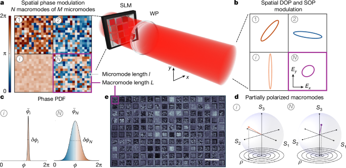
The DOP modulator consists of a phase-only liquid-crystal-on-silicon SLM (Hamamatsu X13138, 1,280 × 1,024 pixels, 12.5 μm pixel pitch, 60 Hz body price) sandwiched between an enter half-waveplate (HWP) and an output pair composed of a quarter-waveplate (QWP) and a HWP. An expanded beam from a continuous-wave laser (λ = 532 nm, 250 mW), with diagonal (D) polarization set by the enter HWP, illuminates the SLM. The output QWP and HWP are mounted on high-speed motorized rotation phases and oriented at angles α and β, that are programmed along with the SLM. The WPs convert the part delay ϕ imparted by a SLM pixel right into a SOP set by (ϕ, α, β), as detailed in Supplementary Observe 1. The DOP and SOP of a macromode are managed by means of the 4 parameters (δϕ, (bar{phi }), α, β). Within the two-SLM implementation (Supplementary Fig. 4), two equivalent SLMs (Hamamatsu X15213-16L, 1,280 × 1,024 pixels, 12.5 μm pixel pitch, 60 Hz body price) are cascaded pixel-to-pixel by the use of a 4f lens system with an inserted HWP at a hard and fast angle γ = 22.5°. The modulator is calibrated utilizing polarimetry measurements carried out by a rotating-WP polarimeter (Thorlabs PAX1000VIS, 0.25° accuracy) that measures S1, S2, S3 and ρ.
Spatial modulation of the DOP and SOP is realized in two completely different configurations. Within the first, the modulated beam is noticed in a far-field aircraft situated at a distance z from the SLM, whereas within the second, it’s noticed within the Fourier aircraft. We element right here the primary configuration, because the experimental set-up is extra versatile and doesn’t require additional optical parts, and the Fourier implementation by the use of a microlens array is detailed in Supplementary Observe 6. The working distance z is ready in line with the micromode dimension l, which determines the diffraction size after which micromodes combine by propagation. At full decision (N = 32 × 32), z is ready to roughly 5 cm. For this z, the dimensions of the macromode shaped within the far discipline is comparable with its dimension L on the SLM.
The modulator is validated by a non-full-Stokes polarization digicam (methodology 1) and a full-Stokes imaging system (methodology 2). The polarization digicam (Thorlabs Kiralux, 2,448 × 2,048 pixels) acquires photos (Fig. 3) of the linear polarization diploma (nu =sqrt{{S}_{1}^{2}+{S}_{2}^{2}}/{S}_{0}), azimuth θ = arctan(S2/S1)/2 and depth S0(x, y). Full-Stokes and DOP imaging is carried out by finishing up Stokes measurements with the digicam in depth mode, that’s, sequentially buying depth projections of the beam profile by means of a QWP and a polarizer at completely different orientations54. The accuracy of the spatial DOP and SOP modulation is evaluated by the ({rm{RMSE}}=frac{1}{N}{sum }_{i}^{N}sqrt{{sum }_{ok}|{S}_{ok}^{{rm{m}}}-{S}_{ok}^{{rm{p}}}^{2}/3}), by which superscripts ‘m’ and ‘p’ denote measured and programmed values, respectively.
Programming the spatial DOP modulator
The SLM lively space is split into N sq. macromodes (blocks of pixels). A macromode is additional divided into M sq. micromodes, every consisting of l × l pixels, with l correctly set to fill the SLM lively space for a goal decision N. For example, we use l = 12 pixels for M = 256 and N = 25 (Fig. 3d), that’s, the micromode dimension is 150 μm on this case. The minimal macromode dimension required for correct spatial modulation of the DOP and SOP is L = 25 pixels, achieved through the use of M = 25 micromodes of size l = 5 pixels (Fig. 3h). For prime-resolution modulation (Fig. 3i), just a few clean pixels of fixed polarization are used to separate the macromodes and keep away from their overlap owing to diffraction. The part masks is constructed by assigning to all of the pixels of the jth micromode a relentless part ϕj within the interval [0, 2π]. The worth ϕj is randomly extracted from a Gaussian PDF that characterizes the ith macromode, ({{mathcal{N}}}^{(i)}(phi )=(1/sqrt{2{rm{pi }}delta {phi }_{i}^{2}})exp [-{(phi -{bar{phi }}_{i})}^{2}/2delta {phi }_{i}^{2}],) with normal deviation δϕi in [0, π/2] and imply ({bar{phi }}_{i}) in [0, 2π]. By various (bar{phi }), the SOP spans a trajectory on the Poincaré sphere that’s tunable by the WP angles.
We calibrate the modulator by performing the evaluation in Fig. 2 at completely different values of (δϕ, (bar{phi }), α, β). In Fig. 2, every knowledge level corresponds to a single-mask experiment. Observe that, as ρ tends to zero, the polarized part turns into much less particular and, persistently, the measurement error on the Stokes parameters is bigger. Averaging over a number of statistically equal masks permits us to scale back the noise noticed in single-mask experiments (Supplementary Fig. 2). The DOP is calibrated utilizing the typical modulation and the becoming operate ρ = aexp(−bδϕ2) + c. The measured SOP (Fig. 2b) is in shut settlement with the polarization matrix mannequin (Supplementary Observe 2). We then assemble a mapping between (S1, S2, S3, ρ) and the 4 parameters (δϕ, (bar{phi }), α, β) = X. A goal beam, spatially modulated in DOP and SOP, is generated by setting the vectors X(i) accordingly. We research the dependence on the variety of micromodes M in Supplementary Fig. 3. Within the two-SLM implementation, the WP angles α and β are changed by a second tunable part ({phi }_{2}^{(i)}), which is ready independently for every macromode and stays fixed inside it. On this case, the modulator is programmed by the vectors ({X}^{(i)}=(delta phi ,bar{phi },{phi }_{2})). The calibration of the two-SLM modulator is reported in Supplementary Fig. 5. The modulator is programmed utilizing customized MATLAB codes.
Avoiding macromode crosstalk
To regulate the spatial modulation of the DOP and SOP, it’s essential that macromodes don’t work together with one another. Any macromode crosstalk would degrade the modulation accuracy, because the state programmed on a macromode would have an effect on its neighbours. To keep away from macromode crosstalk, the far-field distance z have to be chosen appropriately. Because the interplay between two shut micromodes and two shut macromodes happens at a distance on the order of their diffraction lengths zl = πl2/λ and zL = πL2/λ, respectively, the working distance should fulfill zl ≪ z ≪ zL. This situation is achieved simply for big macromodes (l ≪ L). For example, L = 2.4 mm and l = 150 μm, as in Fig. 3d–f, yield roughly 0.1 m < z < 10 m. On this case, macromode crosstalk has a negligible impact. It turns into related when L and l are nearer in worth, as happens when decreasing M to maximise the variety of addressable macromodes. On this case, crosstalk is prevented through the use of just a few clean pixels that spatially separate adjoining macromodes. The size of this buffer space is chosen in order that micromodes on the fringe of two adjoining macromodes don’t have any spatial overlap on propagation. The residual crosstalk is experimentally quantified in Supplementary Observe 9. In Fig. 3i, by which l = 60 μm and z = 5 cm, we use d = 6 clean pixels. Within the Fourier-plane implementation, macromode crosstalk is prevented by design as a result of every microlens operates on a single macromode. This configuration is preferable for purposes that require targeted DOP-modulated gentle.
Encoding colors in polarization
To encode real RGB colors in polarization, SOP modulation alone will not be adequate. In truth, though we might affiliate some colors to completely different SOPs, such a mapping to the sphere floor doesn’t protect the important property that offers any color as a linear mixture of the primaries. To beat this limitation, DOP modulation is critical. We use the map illustrated in Fig. 4a, given by ({S}_{1}=(2{rm{R}}-1)/sqrt{3}), ({S}_{2}=(2{rm{G}}-1)/sqrt{3}) and ({S}_{3}=(2{rm{B}}-1)/sqrt{3}), with R, G, B ∈ [0, 1]. Observe that many different maps are attainable, together with transformations that use a nonlinear relation or the spherical coordinates [θ, χ, ρ] on the Poincaré sphere. We will encode RGB colors with a precision of as much as 8 bits per channel, decided by the SLM bit depth.
Excessive-dimensional PNN
The optical a part of the PNN consists of n optical random layers shaped by a stack of n diffusers (Thorlabs N-BK7 Floor Glass Diffusers with 120-, 200-, 600- or 1,500-grit polishes) and an optoelectronic layer applied by a complementary steel–oxide–semiconductor (CMOS) digicam (Basler a2A1920-160umPRO, 1,920 × 1,200 pixels, 12-bit pixel depth) positioned 10 cm away from the stack of diffusers. A 4 × 4-pixel binning is carried out immediately on the CMOS sensor, which implements a mean pooling layer immediately in {hardware}. The 300 × 300 acquired depth values (12-bit precision) type the enter to a digital backend. The digital community is a few-node community product of two absolutely related layers with 40 hidden nodes and ten output nodes (output lessons). The category is assigned by the softmax operation on the output vector and coaching is carried out through the use of the Adam optimizer.
We classify color photos from the CIFAR-10 dataset53, which consists of 60,000 32 × 32 RGB photos of ten object lessons with 6,000 photos per class. These are divided into 50,000 coaching samples and 10,000 check samples. For comparability, we additionally classify the corresponding greyscale photos obtained by changing the unique RGB dataset. Pictures are polarization-encoded into N = 32 × 32 macromodes of dimension L = 25 pixels (Fig. 4c). The RGB to Stokes mapping in Fig. 4a is used. This performs a nonlinear operation on the enter knowledge. Observe that part encoding can also be nonlinear55. Subsequently, the enter nonlinearity has a minor position within the noticed efficiency enhancement. Classification accuracy is averaged over repeated coaching and testing runs.
We mannequin the high-dimensional PNN by way of cascaded VTMs and partially coherent propagation56, as detailed in Supplementary Observe 7.
Scalability
As a high-dimensional encoder, the spatial DOP modulator helps a decision that scales linearly with the variety of SLM pixels, N = ξ−1npx, with ξ = L2 = M × l2 a set-up-dependent fixed issue (Supplementary Desk 1 studies a comparability of spatial optical encoders in PNNs). In our implementation with 32 × 32 macromodes, ξ ≈ 6 × 10² (Fig. 3h). In accordance with this worth, greater than 10,000 macromodes might be generated with ultrahigh-definition SLMs (4K, npx = 4,160 × 2,464). Subsequently, a large-scale implementation is instantly achievable with off-the-shelf parts.
Multidimensional optical encryption system
Speckle-based encryption of polarization-encoded RGB photos is carried out utilizing a 120-grit ground-glass diffuser as a scattering medium positioned within the focal aircraft of a lens (250 mm focal size), with the transmitted speckle sample (ciphertext) collected by the CMOS digicam. The speckle depth is immediately associated to the enter SOPs by means of the transmission tensor57 of the diffuser. The acquired depth photos (1,200 × 1,200 pixels, 4,096 depth ranges) are downsampled to type a vector of dimension 1 × 90,000. The DNN consists of two absolutely related layers, with w × N hidden nodes and three × N output nodes, related by the use of batch normalization and ReLU activation. The hyperparameter w units the hidden-layer dimension and is tuned to optimize the decryption accuracy (w = 4 for the ends in Fig. 5). The three × N output vector accommodates the values S1, S2 and S3 of the N macromodes. The decrypted picture is obtained by inverse mapping to the RGB values with the chosen relation [R, G, B] ↔ [S1, S2, S3]. The error owing to an incorrect map (safety key) is proven in Supplementary Fig. 17.
The decryption DNN utilized in Fig. 5 has almost 3.8 × 10⁸ learnable parameters (12.2 Gbit at 32-bit precision). It’s skilled on a dataset of 20,000 plaintext–ciphertext pairs. The constancy of the decrypted picture is quantified by the PCC, an simply interpretable metric. We will encrypt any RGB picture as much as 32 × 32 pixels. In Fig. 5, we encrypt CIFAR-10 photos to exhibit operation on the most supported decision.