Simulation-informed kernel-based regression models for predicting temperature distribution in microwave hyperthermia

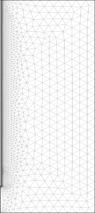
The spatial temperature subject was first obtained by numerically fixing the coupled bioheat downside over the computational area. As illustrated in Fig. 5, the best temperatures happen within the area instantly surrounding the antenna, the place electromagnetic power deposition is strongest. This localized heating sample displays the supposed habits of the microwave applicator, with thermal depth concentrated close to the therapy area moderately than distributed uniformly all through the encircling tissue. The ensuing temperature subject is inherently depending on the working circumstances of the heating system, and variations in parameters such because the electromagnetic subject energy can modify each the magnitude and spatial extent of the generated warmth.

The simulation-derived temperature knowledge have been then used to develop and assess the machine-learning surrogate fashions. Kernel Ridge Regression (KRR), Help Vector Machine (SVM), and Relevance Vector Machine (RVM) have been educated to estimate temperature T from the radial and axial coordinates (r, z). The tunable parameters of every mannequin have been optimized utilizing the Cuckoo Search (CS) algorithm. Their predictive capabilities have been subsequently evaluated towards the numerical-simulation outcomes utilizing a typical set of efficiency standards, permitting the relative accuracy, robustness, and limitations of the three regression approaches to be in contrast systematically.

Mannequin efficiency was evaluated utilizing the coefficient of dedication R², imply squared error (MSE), imply absolute error (MAE), and most absolute error. These metrics have been calculated utilizing their normal formulations¹⁸:

the place (:{T}_{i}) and (:{widehat{T}}_{i}) denote the numerical-simulation temperature and the corresponding mannequin prediction, respectively, (:stackrel{-}{T}) is the imply noticed temperature, and n is the variety of evaluated samples. Greater R and decrease MSE, MAE, and most error point out higher predictive efficiency.

Temperature distribution within the area (Ok) calculated utilizing numerical simulation.

From a therapy perspective, the expected temperature subject ought to be interpreted in relation to clinically related thermal thresholds. Typical hyperthermia goals to raise tumor temperature to roughly 45 °C (about 318 Ok) whereas limiting extreme heating of surrounding tissue³. The numerical temperature subject used within the current examine spans roughly 310–355 Ok, indicating that some areas, notably close to the antenna, attain temperatures considerably above the standard hyperthermia vary. These high-temperature areas ought to due to this fact be interpreted as potential localized overheating or ablative zones moderately than as the specified temperature all through the handled tissue. On this context, the surrogate mannequin can help in quickly figuring out the spatial distribution of temperature and areas approaching or exceeding the supposed thermal vary. Nonetheless, the current mannequin shouldn’t be interpreted as a medical management system, since patient-specific security margins and potential medical validation weren’t investigated on this examine. The localized temperature most noticed close to the microwave antenna is in line with the thermal sample reported by Yang et al., who equally noticed the best tissue temperatures adjoining to the applicator adopted by a progressive lower with growing distance¹⁵. This settlement helps the bodily consistency of the spatial temperature sample obtained within the current simulation.

The cross-validation normal deviations present a further indication of the steadiness of the evaluated fashions throughout folds. Particularly, the comparatively small normal deviations noticed for KRR, SVM, and RVM point out restricted variation in predictive efficiency throughout the 5 validation subsets. Among the many evaluated fashions, SVM exhibited the smallest cross-validation normal deviation (0.0006289), supporting the consistency of its predictive efficiency. These cross-validation statistics have been interpreted along with the impartial test-set MSE, MAE, and most absolute error to keep away from counting on a single efficiency measure.

The mannequin choice was primarily based on a complete comparability of predictive accuracy and generalization efficiency. The first criterion was the coefficient of dedication (R²) obtained on the impartial check dataset, with the next R² indicating higher predictive functionality. This criterion was complemented by the error-based metrics, together with imply squared error (MSE), imply absolute error (MAE), and most absolute error, for which decrease values have been most popular. To evaluate the steadiness and generalization consistency of the fashions, the imply and normal deviation of the R² values obtained from 5-fold cross-validation have been additionally thought of. Accordingly, the ultimate mannequin was chosen by collectively contemplating excessive check R², low prediction errors, excessive cross-validation imply R², and low cross-validation variability moderately than counting on a single efficiency indicator.

The outcomes of ML modeling and their comparisons are listed in Tables 2 and 3 for the three fashions employed on this examine. Based mostly on the predefined mannequin choice standards, the fashions have been in contrast in line with their impartial check R², prediction error metrics, and 5-fold cross-validation efficiency. The outcomes display the superior total efficiency of SVM. It displays the best R² scores for each the coaching and testing datasets, in addition to the best cross-validation imply. Moreover, SVM achieves the bottom MSE and MAE amongst all fashions, indicating superior total predictive accuracy. Though RVM displays a decrease most error than SVM, the choice was primarily based on the collective evaluation of all predefined standards moderately than on most error alone. Contemplating its increased check R², decrease total prediction errors, and robust and steady cross-validation efficiency, SVM was chosen as the popular mannequin for predicting temperature primarily based on spatial coordinates.

A direct wall-clock comparability between the COMSOL simulation and the machine-learning fashions was not recorded through the authentic computational runs. As a result of computational time relies upon strongly on the {hardware} configuration, solver settings, software program implementation, and model-specific parameters, retrospective numerical estimates wouldn’t present a dependable or reproducible benchmark. Within the current framework, the COMSOL finite-element simulation represents the physics-based computational stage used to generate the temperature subject, whereas coaching of the surrogate fashions is carried out offline utilizing the ensuing simulation knowledge. As soon as educated, the surrogate fashions consider the temperature response straight from the spatial coordinates with out repeatedly fixing the coupled bioheat and electromagnetic equations. Due to this fact, their principal computational benefit is anticipated throughout repeated prediction, though no quantitative speed-up issue is claimed within the current examine. A managed runtime comparability carried out on similar {hardware} is recognized as an essential course for future work.

Whereas KRR and RVM additionally exhibit aggressive efficiency, SVM offers one of the best total efficiency primarily based on its increased R², decrease MSE and MAE, and steady cross-validation outcomes. RVM, nonetheless, achieves the bottom most absolute error among the many evaluated fashions.

Though the SVM achieved a comparatively low total MAE of 0.893 Ok, its most absolute error reached 12.23 Ok. This distinction is clinically essential as a result of a low common error doesn’t exclude bigger native deviations in particular person areas. Consequently, the current surrogate ought to be thought of a temperature-prediction device requiring additional validation earlier than software to therapy management or safety-critical resolution making.

The current comparability is restricted to the three investigated kernel-based surrogate fashions. Due to this fact, the reported superiority of SVM ought to be interpreted solely relative to KRR and RVM throughout the current dataset and simulation setting. Future work ought to lengthen the benchmarking to less complicated statistical baselines and different machine-learning households, akin to linear regression, tree-based regressors, and neural-network fashions.

Distribution of errors in check dataset for SVM mannequin.

Based mostly on the great analysis of R² scores and error charges, the Help Vector Machine emerges because the optimum mannequin for predicting temperatures within the given system. Distribution of residuals for this mannequin are proven in Fig. 6. This mannequin achieved the best R² scores (coaching: 0.9766, testing: 0.9768), signifying a sturdy match to the info, together with the bottom error charges, comprising MSE (3.6647E + 00) and MAE (8.9252E-01), showcasing correct predictions. RVM achieved the smallest most error (9.3946 Ok), whereas SVM confirmed one of the best total efficiency primarily based on its increased R² and decrease MSE and MAE. The residual distribution proven in Fig. 6 offers a further diagnostic view of the chosen SVM mannequin past the tabulated error metrics. Along with the reported MSE, MAE, and most absolute error, this residual evaluation helps characterize the unfold of prediction errors on the impartial check set. Extra detailed visualization instruments, akin to parity plots and spatial error maps, could additional improve efficiency evaluation and are due to this fact recognized as helpful extensions for future work.

Characteristic significance evaluation for the dataset is indicated in Figs. 7, 8 and 9, the place it’s noticed that the axial coordinate (z) has a larger affect on temperature than the radial coordinate (r). Whereas this rating is in line with the correlation construction reported in Fig. 2 (|r|: z–T = 0.64 vs. r–T = 0.39), it’s corroborated right here by the educated SVM surrogate itself moderately than the uncooked knowledge alone, since Fig. 7 displays the sensitivity of the fitted mannequin’s predictions moderately than a easy correlation coefficient. To additional probe mannequin interpretability past this world rating, Figs. 10 and 11 current one-dimensional partial dependence plots, exhibiting the expected temperature as a perform of r and z respectively, with the complementary coordinate held at consultant fastened values. These partial dependence curves reveal the practical type of every variable’s impact — together with native nonlinearities and the placement of most sensitivity alongside every axis — {that a} single significance rating can not seize. As well as, the native gradients of predicted temperature with respect to r and z (∂T̂/∂r, ∂T̂/∂z), estimated numerically from the educated SVM mannequin throughout the area, affirm that the biggest sensitivity to z happens close to the antenna tip area, in line with the placement of peak predicted temperature proven in Figs. 8 and 9. Furthermore, 3D and 2D illustrations of temperature distribution are proven in Figs. 8, 9, 10 and 11. These outcomes have been constructed utilizing ML fashions and present nice settlement with the numerical simulations. In each 3D and 2D illustrations, the area with the utmost T could be noticed precisely. The spatial sample reconstructed by the surrogate mannequin can be in line with earlier microwave-hyperthermia modelling, the place peak temperatures have been concentrated close to the antenna and decreased towards extra distant tissue areas¹⁵.

Characteristic significance of enter coordinates.

Three-dimensional visualization of the expected temperature subject as a perform of the radial and axial coordinates, r and z.

Contour map illustrating the spatial distribution of the expected temperature throughout the computational area.

Remoted affect of the radial coordinate, r, on the expected temperature response.

Remoted affect of the axial coordinate, z, on the expected temperature response.