Enhancing groundwater potential mapping in arid regions through integrated microwave remote sensing, statistical analysis, and geophysical-based modeling

Determine 4 illustrates the structured workflow of the built-in methodology utilized on this research. The groundwater-potential (GwP) evaluation combines topographic, geological, structural, hydrogeological, and climatic variables inside a hybrid statistical framework. To additional refine the evaluation, the strategy incorporates information from DC-resistivity soundings and aeromagnetic surveys. The following sections describe every methodological step intimately.

The Detailed methodology flowchart reveals the integrative framework, together with distant sensing and geophysical dataset evaluation for enhancing the groundwater potential mapping.

Datasets assortment and preparation

The first information sources embody S1A VV and VH polarization imagery obtained from the Alaska Satellite tv for pc Facility for lineament extraction and Rb extraction, the ALOS-DEM for topographic and hydrogeological parameter extraction, and IMERG information for rainfall distribution evaluation. Further datasets comprise groundwater effectively areas and a lithological map derived from the CONOCO⁵⁹ database offered by the European Soil Information Heart (https://esdac.jrc.ec.europa.eu/content/geologic-map-egypt). All digital datasets have been geometrically corrected and co-registered to the Common Transverse Mercator (UTM) coordinate system, WGS 1984 Zone 36N, utilizing ArcGIS Professional 3.6⁶². The following sections present an in-depth evaluation of the dependent stock and unbiased issue datasets, emphasizing their significance throughout the modeling framework. Desk 1 summarizes all datasets used on this research, together with the supply, acquisition date, native decision, preprocessing steps, and the ultimate coordinate reference system to which all layers have been standardized.

Potential controlling elements

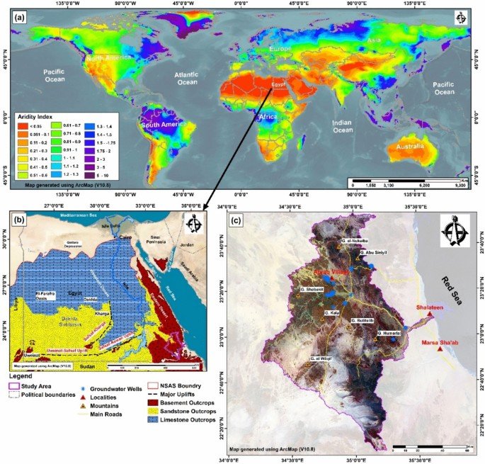
Aly et al.⁶⁴ emphasised that making ready thematic information layers and choosing related elements are important parts of any modeling strategy. On this research, ten thematic parameters have been recognized to evaluate groundwater potential throughout the SCAq area, as they both affect or exhibit correlations with groundwater prevalence^{8,24,48,50,60}. These parameters embody slope, curvature, Topographic Wetness Index (TWI), Stream Density (SD), Distance to Stream (DTS), lithology, Radar backscattering (Rb), Lineament Density (LD), Lineament-Stream Intersection Density (LSID), and Common Annual Rainfall (AAR).

The choice standards for these parameters are grounded in in depth literature that highlights their relevance to groundwater potential within the SCAq area, notably within the context of the Jap Desert’s advanced terrain^50,60. The regional geology options various lithological formations formed by prevalent faults and fractures, as evidenced by the linear boundaries of rock items (Fig. 3). These geological traits play a vital function in influencing groundwater storage and motion, affecting aquifer recharge dynamics.

Moreover, hydrological elements resembling Distance to Stream (DTS), Stream Density (SD), and the Topographic Wetness Index (TWI) are important for figuring out potential groundwater accumulation zones^65,66. In response to Sahour et al.⁶⁵, areas in proximity to pure drainage techniques inside watersheds are likely to exhibit shallower groundwater tables, that are important for sustainable water sources. On this means, these parameters collectively inform our understanding of groundwater conduct and improve the reliability of our modeling strategy.

Topographic elements

Key topographic parameters, notably slope and curvature, play a important function in aquifer recharge, particularly within the extremely skilled terrains of the Jap Desert. These parameters have been derived from an ALOS/PALSAR-1 Radiometrically Terrain-Corrected (RTC) digital elevation mannequin (DEM) product, acquired on June 11, 2009, by the Alaska Satellite tv for pc Facility (ASF)⁶⁷. The dataset includes twelve scenes in Wonderful Beam Single (FBS) polarization mode (HH), every with a local spatial decision of 12.5 m. All scenes have been downloaded in GeoTIFF format, mosaicked utilizing the “Mosaic to New Raster” instrument in ArcGIS Professional 3.6, and projected to the Common Transverse Mercator (UTM) Zone 36N coordinate system with the World Geodetic System 1984 (WGS84) datum.

The spatial distribution of floor slope was calculated utilizing the Slope instrument (ArcGIS Professional V3.6), which calculates the utmost fee of change in elevation between every cell and its eight neighbors. The output slope grid was computed in levels. This parameter is crucial for understanding how water strikes throughout the panorama. Moreover, the Curvature instrument was utilized to evaluate deviations from a planar floor, producing an output grid the place detrimental values signify concave, constructive values signify convex, and 0 values signify flat surfaces. These topographical options considerably affect hydrological processes, figuring out areas of water accumulation and influencing the effectivity of aquifer recharge.

Hydrological elements

Hydrological elements, together with DTS, SD, and TWI, provide important insights into potential groundwater accumulation zones⁶⁶. Consequently, the mosaicked 12.5 m ALOS-DEM was used as enter for hydrological evaluation. Areas in proximity to pure drainage techniques inside watersheds usually tend to exhibit a shallow groundwater desk⁶⁵. Consequently, ALOS-DEM information have been used to extract the pure drainage community maps. The spatial distribution of stream networks was obtained by making use of the eight-direction (D-8) movement algorithm⁶⁸ utilizing the Arc Hydro toolset (model 2.0) in ArcMap. The stream community was delineated utilizing a flow-accumulation threshold of 2000 pixels, such that solely cells draining not less than 2000 upstream cells have been included within the community. The SD, outlined because the ratio of complete stream size to drainage basin space, was derived utilizing the Line Density instrument, with a search radius of 1000 m and an output cell measurement of 10 m. The TWI is broadly used to evaluate soil moisture distribution and saturation zones inside a given terrain⁶⁹. The TWI was computed utilizing the next Eq. (1), applied within the ArcGIS Raster Calculator.

the place (a) is the native upslope contributing space (m²/m), (b) is the slope gradient (measured in levels) at that particular place, and “ln” is a continuing that refers back to the Napierian logarithm.

Geological elements

The variations in floor geology and soil distribution immediately have an effect on hydrological processes, figuring out how successfully water infiltrates into the bottom and replenishes aquifers. Every rock kind possesses distinct properties that considerably affect floor water motion and soil porosity throughout the basins. The lithological map used on this evaluation was derived from the revealed geological map of CONOCO⁵⁹, scaled at 1:500,000 (Fig. 3). The geological map was scanned, georeferenced in ArcGIS utilizing floor management factors, and the geological polygons have been digitized. This thematic vector layer was then transformed to raster format at a ten m cell measurement utilizing the Polygon to Raster instrument to standardize the layer, facilitating the project of weights and ranks.

Lineaments, noticed as linear or curvilinear options in satellite tv for pc imagery, embody geological buildings resembling faults, fractures, and joints, taking part in a vital function in groundwater movement and accumulation²⁷. Two high-resolution Floor Vary Detected (GRD) scenes from S1A VV and VH polarizations, acquired in June 2021 utilizing the Interferometric Huge (IW) mode, have been used because of the availability of the photographs over the entire basin without charge (Supply of knowledge). These pictures have been captured in a descending orbit with a spatial decision of 10 m × 10 m. The preprocessing included making use of the orbit file, speckle filtering, radiometric calibration, thermal noise elimination, and Vary-Doppler Terrain Correction. The pictures have been subsequently transformed to a decibel scale to mitigate disturbances within the VV and VH bands. A 3 × 3 Lee filter was utilized to reduce speckle noise whereas preserving structural integrity, notably in homogeneous areas and alongside characteristic boundaries^70,71.

Lineaments, noticed as linear or curvilinear options in satellite tv for pc imagery, embody geological buildings resembling faults, fractures, and joints²⁷. For his or her extraction, two high-resolution Floor Vary Detected (GRD) scenes from Sentinel-1A (S1A) with VV and VH polarizations have been acquired. The scenes, captured on June 21, 2021, in Interferometric Huge (IW) mode with a descending orbit, have been downloaded from the Alaska Satellite tv for pc Facility (ASF) vertex portal. Every scene had a local spatial decision of 10 m × 10 m. Preprocessing was carried out utilizing the Sentinel-1 Toolbox in SNAP (ESA SNAP 9.0) and included: (1) Apply Orbit File, (2) Thermal Noise Elimination, (3) Radiometric Calibration to sigma0, (4) Vary-Doppler Terrain Correction utilizing the SRTM 30 m DEM, and (5) Conversion to decibel (dB) scale. To mitigate speckle noise whereas preserving structural integrity, a 3 × 3 Lee filter was utilized to the calibrated dB pictures^70,71.

Lineament extraction was carried out utilizing the LINE module in CATALYST PROFESSIONAL PCI Geomatica 2022 (model 23.0). The filtered VV polarization dB picture was used as enter. The next parameter values have been set for the extraction algorithm, with GTHR and ATHR adjusted from default values to reinforce geological characteristic detection, following Embaby et al.⁸

The extracted vector lineaments have been manually reviewed and edited to take away non-geological options (e.g., roads, discipline boundaries). The Intersect instrument in ArcGIS was subsequently utilized to find out intersection factors between the extracted lineaments and stream networks. Structural indices, together with LD and LSID, have been computed utilizing the Kernel Density instrument in ArcGIS Professional V3.6 with a search radius of 1000 m and an output cell measurement of 10 m.

Radar backscatter depth has been well known as an efficient parameter for monitoring hydrological parts^72,73. A static regional Rb picture was generated from the preprocessed S1A VH polarization dB picture. The picture was resampled to a ten m grid to research spatial variations in soil properties.

Climatic elements (common annual rainfall)

Rainfall serves as the first water supply in arid and semi-arid basins⁷⁴. Every day precipitation information have been acquired from the NASA World Precipitation Measurement (GPM) mission’s Built-in Multi-satellitE Retrievals for GPM (IMERG) Last Run product (Model 06). The info have been accessed by way of the NASA Giovanni platform (https://giovanni.gsfc.nasa.gov/giovanni/) for the interval from January 1, 1998, to January 31, 2019⁷⁵. This dataset gives half-hourly precipitation estimates at a local spatial decision of 0.1° × 0.1° (roughly 10 km × 10 km). The every day information have been aggregated to month-to-month, then to annual totals. A protracted-term Common Annual Rainfall (AAR) grid was computed by averaging the 21 annual grids. This coarse AAR raster was then projected to UTM Zone 36N, WGS84, and interpolated to a ten m grid cell measurement to match different thematic layers utilizing the Inverse Distance Weighting (IDW) geostatistical methodology in ArcGIS, with an influence parameter of two and a variable search radius. AAR was recognized as a related conditioning issue, given its applicability over in depth spatial scales⁷⁵.

Groundwater stock information

The residents make the most of springs, the place pure groundwater is discharged from the NSAS⁴⁹, together with drilled groundwater wells for every day use and agricultural actions⁴⁵. A complete of 40 productive groundwater (PGw) factors, together with productive effectively websites and some spring areas, have been recognized utilizing Google Earth Professional imagery and discipline observations throughout the research space. To fulfill the presence/absence necessities of the bivariate fashions and enhance information distribution, absence factors have been generated from two complementary sources: (1) documented dry wells (shallow, non-productive boreholes) encountered within the discipline, and (2) bedrock exposures and high-terrain areas recognized from satellite tv for pc imagery and geological maps, that are characterised by excessive runoff and minimal overburden, making them inherently unfavorable for groundwater storage. To account for the affect of native faults and aquifer discontinuities, a 100-m buffer zone was established round all presence factors. No absence factors have been sampled inside these buffers to stop battle with productive structural areas.

For modeling, 28 PGw factors (70%) and an equal variety of absence factors have been randomly chosen for coaching the WOE and EBF fashions, whereas the remaining 12 PGw factors (30%) have been reserved for validation. Last unbiased validation was carried out utilizing 17 Vertical Electrical Sounding (VES) factors, which have been excluded from the coaching course of solely.

Hybrid GIS-based bivariate evaluation for groundwater potential mapping

Deciding on an applicable resolution rule is essential, because it determines the rating and weighting methodology used to combine the influencing elements underneath predefined weights, thereby considerably affecting the evaluation outcomes. This research employed two bivariate geospatial fashions, Weight of Proof (WoE) and Evidential Perception Perform (EBF), to guage the rating of sub-class elements throughout the investigated basin.

All raster layers, apart from lithology and curvature, have been reclassified into 5 scoring ranges utilizing the pure breaks (Jenks) classification methodology, which operates at a spatial decision of 12.5 m. This classification strategy enhances differentiation amongst lessons by figuring out optimum threshold values that group comparable information factors based mostly on inherent patterns. The ensuing framework successfully represents the various topographic, geological, structural, hydrogeological, and climatic traits of the research space, every of which performs a task in influencing the spatial distribution of groundwater potential (GwP) inside SCAq.

To look at the intricate relationships between dependent and unbiased controlling elements, 70% of the groundwater stock factors have been utilized. The Index of Entropy (IOE) methodology was deployed to assign weights to the conditioning elements affecting GwP. Moreover, a hybrid modeling framework was developed by integrating IOE with WoE and the EBF methodology to generate predictive GwP maps.

The ensuing groundwater potential fashions have been subsequently validated utilizing the Space Beneath the Curve (AUC) strategy, with the remaining 30% of the dataset employed for mannequin reliability evaluation. These fashions have been developed utilizing the Spatial Information Modeller (SDM) extension in ArcMap 10.8, together with XLSTAT and IBM SPSS Statistics. A complete description of the adopted methodology is offered within the subsequent sections.

Index of entropy (IOE) mannequin

The Index of Entropy (IOE) methodology is usually employed to evaluate the uncertainty and instability of a system⁷⁶. On this research, the IOE was utilized to find out the predictive weights (({textual content{W}}_{textual content{j}})) of every controlling issue based mostly on the next equations⁷⁶.

the place the frequency ratio (FR) quantifies the spatial affiliation between a particular issue class and the goal phenomenon. For a given groundwater issue, (A) represents the world of a particular class inside that issue, whereas (B) is the full space of your entire issue. Equally, (C) denotes the variety of pixels in that class space, and (D) is the full variety of pixels within the research space. The time period (b) is the share space of a particular class relative to the issue’s complete space, whereas (a) is the share space of the issue relative to your entire research area. The chance density is denoted by Pij. Entropy values are expressed as H_j (precise entropy for issue j) and H_jmax (most potential entropy for that issue). S_j is the variety of lessons inside issue j, I_j is the knowledge coefficient reflecting the issue’s predictive energy, and w_j is the resultant weight worth assigned to the issue as an entire, which ranges between 0 and 1.

GWP map of the entropy methodology was ready by overlaying all of the thematic layers by way of the obtained weights of every mannequin by the spatial evaluation instrument within the ArcGIS bundle utilizing the next equation:

the place GWP is the groundwater potential zone; Wi is every layer weight and Ri the category charges inside a thematic layer.

Weight of proof (WOE) mannequin

The Weight of Proof (WoE) mannequin is a data-driven, Bayesian methodology that estimates the chance of groundwater prevalence given a particular evidential class. For every class, it computes two weights: a constructive weight (W⁺) when the category is current and a detrimental weight (W⁻) when it’s absent. The distinction, C = W⁺ − W⁻, summarizes the category’s total spatial affiliation with groundwater; bigger constructive contrasts point out a stronger favorable relationship.

These weights are derived by evaluating the density of presence factors (groundwater occurrences) inside a category to the density of absence factors exterior that class. As a bivariate statistical approach, WoE combines easy logical ratios with Bayesian chance to quantify the proof offered by every issue class for predicting groundwater presence⁷⁷. This produces goal, class-level weights that cut back subjective bias and assist reveal advanced interdependencies amongst conditioning elements⁷⁸. The constructive and detrimental weights for every sub-category are computed utilizing the next equations^79,80.

the place F and (overline{textual content{F} }) signify the presence and absence of conditioning parameters, respectively; P denotes chance; and G, and (overline{textual content{G} }) correspond to the presence and absence of groundwater, respectively.

Customary deviation of W is calculated as follows⁸⁰:

the place S²W⁺ and S²W⁻ are outlined because the variances of constructive weights and detrimental weights, respectively.

The ultimate WOE coefficients (({R}_{WOE})) assigned to every issue class will be obtained as follows.

the place ({W}_{min}^{-}) represents an total measure of spatial affiliation between the coaching factors and the evidential theme, combining the consequences of the 2 weights. Generally, W⁺ will be near zero, but W^– is strongly detrimental. This example arises if the presence of the theme shouldn’t be notably predictive of coaching factors, however the absence of the theme gives robust proof that factors are unlikely to happen. Conversely, there will be an imbalance between absolutely the values of W⁺ and W^– within the different path, or the 2 weights can have absolute values in about the identical vary.

In response to Bonham-Carter⁸⁰, absolutely the values of weights present a measure of predictive energy: values between 0 and 0.5 are mildly predictive; values between 0.5 and 1 are reasonably predictive; values between 1 and a pair of are strongly predictive; and values larger than 2 are extraordinarily predictive.

The ultimate ({GwP}_{textual content{W}textual content{O}textual content{E}-text{I}textual content{O}textual content{E}}) map was generated by making use of the inferred IOE weight (({textual content{W}}_{j})) to the ranked numerical values of issue lessons, represented as attributes of ({R}_{WOE}).

In commonplace WOE, lessons with zero presence or zero absence factors yield infinite or undefined weights, inflicting numerical instability. Within the research space, for instance, the basement bedrock lithological class contained zero productive groundwater factors in comparison with the Nubian Sandstone and Alluvium deposits. To deal with this, a correction issue of 0.5 was added to all presence and absence counts following Bonham-Carter⁸⁰, utilizing the ArcSDM toolbox. This correction yielded a finite detrimental weight (W⁺ = − 1.25) for the basement bedrock class, appropriately indicating unfavorable situations whereas preserving numerical stability.

Evaluation of predictor independence

A elementary assumption of the Weight of Proof mannequin is that evidential themes are conditionally unbiased with respect to the coaching factors⁸⁰. Violation of this assumption can result in overestimation of posterior possibilities and unstable weight estimates⁸¹. To guage the diploma of dependence among the many ten conditioning elements, a multicollinearity evaluation was performed utilizing pairwise Pearson correlation and Variance Inflation Issue (VIF).

Pearson correlation coefficients (r) have been calculated between all issue pairs (Desk S1), with |r|> 0.7 indicating a robust correlation⁸². VIF was computed as VIF = 1/(1 − R²), the place values exceeding 5 point out reasonable multicollinearity considerations (Desk S2)⁸³. Robust correlations have been noticed between bodily coupled pairs: Slope–TWI (r = − 0.82), LD–LSID (r = 0.86), DTS–SD (r = 0.71), and Slope–Rb (r = 0.73). VIF values remained inside acceptable ranges (< 5) for many elements, with LSID displaying a barely elevated worth (5.26) attributable to its correlation with LD. Curvature and Rainfall exhibited weak correlations with all different elements (VIF < 1.3), confirming their unbiased contributions. Regardless of these correlations, all elements have been retained attributable to their conceptual distinctiveness: Slope controls runoff velocity whereas TWI identifies saturation zones; LD displays fracture depth whereas LSID particularly targets permeable fracture intersections^82,83

These correlations mirror the inherent bodily relationships among the many elements relatively than information artifacts. Though all elements have been retained attributable to their conceptual distinctiveness, WOE is thought to be delicate to conditional dependence. To deal with this, the ten elements have been organized into 5 conceptual teams based mostly on their hydrogeological roles: topographic (Slope, TWI, Curvature), structural (LD, LSID), hydrologic (DTS, SD, Rainfall), geologic (Lithology), and floor (Radar backscattering). Inside every group, reasonable to robust correlations are anticipated as a result of the elements seize totally different dimensions of the identical subsurface course of. For instance, LD measures the frequency of lineaments, whereas LSID targets their intersections. Collectively, their mixed contribution extra successfully represents structural management on groundwater movement than both issue alone. Slightly than treating correlated elements as unbiased predictors, this grouping framework interprets their joint contribution as reflecting an built-in hydrogeological course of^82,83.

Evidential perception perform (EBF) mannequin

The Evidential Perception Perform (EBF) is a knowledge-driven spatial modeling framework used right here to evaluate groundwater potential by integrating a number of conditioning elements⁸⁴. On this strategy, thematic layers representing elements that management groundwater prevalence (e.g., lithology, slope, land use) are handled as distinct items of proof. The mannequin then synthesizes this proof to supply predictive groundwater potential maps⁸⁰. This synthesis is achieved by quantifying the spatial correlation between every evidential layer and the areas of present groundwater wells. By evaluating how strongly every issue class is related to effectively presence, the mannequin derives weights that kind the idea for the ultimate integration. This data-driven correlation enhances the objectivity and reliability of the predictive map.

A key benefit of the EBF mannequin is its capability to not solely delineate potential groundwater zones but additionally to explicitly quantify the uncertainty inherent in these predictions⁸⁴. This twin output is especially useful for decision-making, because it gives stakeholders with a measure of confidence within the mapped zones, thereby supporting extra nuanced and efficient groundwater administration methods.

The mannequin is formalized throughout the Dempster-Shafer principle of proof, which generalizes conventional Bayesian possibilities into decrease and higher chance bounds⁸⁵. On this framework, the decrease and higher possibilities correspond to the assumption (Bel) and plausibility (Pls) measures, respectively. The framework additionally explicitly quantifies associated measures, together with the diploma of disbelief (Dis), which represents help in opposition to a proposition, and the diploma of uncertainty (Unc), which displays a lack of expertise or battle between items of proof⁸⁶. Collectively, these 4 features (Bel, Dis, Unc, and Pls) present a complete illustration of the evidential help for groundwater prevalence throughout the research space.

An in depth rationalization of the algorithm is offered by Carranza et al.⁸⁵. Within the context of groundwater potential mapping utilizing EBF^86,87, the body of discernment is outlined by Eqs. (14) and (15):

the place:

λ(Tp)E_ij = Weight of proof for the presence of groundwater given the category (j) of issue (i). This can be a dimensionless ratio.

N (G ∩ E_ij) = Variety of pixels containing groundwater wells that additionally fall inside class (j) of issue (i).

N(G) = Whole variety of groundwater effectively pixels in your entire research space.

N(E_ij) = Whole variety of pixels comprising class (j) of issue (i).

N(C) = Whole variety of pixels in your entire research space.

The idea measure is given by:

The diploma of disbelief is outlined as:

Uncertainty is calculated as:

Plausibility (Pls, representing the utmost potential help for groundwater prevalence. It’s the sum of perception and uncertainty, and is dimensionless. Pls is expressed as:

The ultimate GwP map generated utilizing the EBF-IOE mannequin was obtained by making use of the inferred IOE weight (Wj) to the ranked numerical values of issue lessons represented as attributes of Bel:

The GwP maps have been categorized into 5 susceptibility ranges: very low, low, reasonable, excessive, and really excessive, using the pure breaks classification methodology in ArcMap.

Validation of groundwater potential (GwP) fashions

The validation of GwP fashions was performed utilizing a mix of statistical, spatial, and field-based approaches to make sure strong analysis of predictive efficiency and generalizability. Given the comparatively small dataset and the affect of spatial autocorrelation, a number of complementary validation strategies have been employed.

A repeated k-fold cross-validation (CV) framework was applied to beat the constraints of a single random information cut up. The dataset, comprising 40 productive groundwater factors and 40 absence factors (n = 80), was subjected to five iterations of fivefold CV. In every iteration, the info have been randomly divided into 5 subsets, with 4 folds (64 factors) used for coaching and the remaining fold (16 factors) used for testing. This repeated resampling generated a distribution of efficiency metrics, permitting the computation of imply Space Beneath the Curve (AUC) values and corresponding commonplace deviations, thereby offering a dependable estimate of mannequin accuracy and related uncertainty.

To additional handle the consequences of spatial autocorrelation, spatially blocked cross-validation was utilized as the first check of mannequin generalization. The research space was divided into 5 spatially contiguous blocks based mostly on pure geographic boundaries. Fashions have been iteratively skilled on 4 blocks and evaluated on the remaining block till every block had been used as a check set. Importantly, the spatial blocks used for validation have been outlined independently of the groundwater prevalence clustering employed throughout mannequin growth. The blocked cross-validation was utilized solely throughout mannequin analysis and didn’t affect the technology of coaching samples or the spatial distribution of productive and non-productive groundwater factors. Consequently, the blocked validation gives an unbiased evaluation of mannequin generalization functionality in beforehand unsampled areas and gives a extra conservative estimate of predictive efficiency than typical random cross-validation.

Mannequin discrimination capacity was evaluated utilizing the Receiver Working Attribute (ROC) curve evaluation^30,88. For every validation iteration, ROC curves have been generated by plotting the True Optimistic Charge (TPR; sensitivity) in opposition to the False Optimistic Charge (FPR; 1 − specificity) throughout a variety of classification thresholds. The Space Beneath the ROC Curve (AUC) was calculated utilizing the trapezoidal rule^85,86:

the place TPRi and TPRi + 1 signify the true constructive charges, and FPRi and FPRi + 1 signify the false constructive charges at consecutive threshold values (i) and (i + 1). Last reported AUC values signify the imply throughout all CV iterations with related commonplace deviation. AUC values vary from 0 to 1; values above 0.7 are thought of acceptable, and people above 0.9 point out excellent predictive accuracy⁸⁸.

Along with statistical validation, frequency ratio evaluation was employed to evaluate the spatial settlement between noticed groundwater occurrences and predicted suitability lessons. This analysis was based mostly on two assumptions: (i) excessive and really excessive GwP zones ought to occupy a comparatively smaller proportion of the research space, and (ii) a dependable mannequin ought to assign the bulk (> 50%) of noticed groundwater factors to not less than reasonable suitability zones, with increased concentrations in excessive and really excessive lessons. This spatial validation gives an intuitive measure of mannequin consistency with noticed patterns.

Lastly, unbiased floor reality validation was performed utilizing 17 VES factors and discipline observations from present wells and is derived situated inside excessive and really excessive potential zones. These VES information weren’t included in mannequin coaching, guaranteeing independence of validation. The geophysical information offered important insights into subsurface situations, together with lithological variations, aquifer thickness, depth to bedrock, groundwater ranges, salinity, and structural options resembling faults and fractures.

To additional help mannequin validation, detailed geophysical investigations have been carried out in excessive and really excessive GwP zones of Wadi Hodein. The combination of aeromagnetic information and VES measurements enabled the identification of subsurface lithological variations and structurally managed aquifer techniques. Aeromagnetic information delineated faults and fractures, whereas VES information characterised resistivity variations related to groundwater saturation and salinity. The robust settlement between geophysical proof and predicted high-potential zones confirms the reliability of the GwP fashions in figuring out structurally managed groundwater techniques.

Geophysical investigations

Detailed geophysical investigations have been performed throughout the excessive and really excessive GwP and the encompassing zones of Wadi Hodein to evaluate the function of subsurface buildings in controlling aquifer techniques (Fig. 5a). Drilled wells and pure springs present vital variability in depth, yield, and water high quality over brief distances, reflecting the complexity of the subsurface and the presence of various aquifer techniques.

Geophysical Datasets within the Recognized Excessive Potential Zone: (a) Aeromagnetic survey space and areas of land-based Vertical Electrical Sounding (VES); (b) A zoomed-in map of VES factors, geoelectrical cross-sections, and drilled wells; (c) Calibration of resistivity interpretation of VES12 alongside the lithologic log of a drilled effectively.at Wadi Dif. These figures have been ready utilizing ArcGIS Professional v3.6 (https://www.esri.com/en-us/arcgis/products/arcgis-pro/overview). The VES curve interpretation was generated utilizing IPI2win free software program accessible at http://geophys01.geol.msu.ru/ipi2win.htm.

A DC resistivity survey (17 VESs) was deliberately focused inside these zones to deal with subsurface complexities, particularly fault impacts and basement reduction, that distant sensing and WOE modeling can not absolutely seize. Low-potential zones weren’t surveyed attributable to logistical constraints and the targeted aim of validating high-potential targets.

To beat the floor limitations of distant sensing and RadarSat, aeromagnetic and VES information have been built-in. Aeromagnetic information delineated lithological variations and structural options (faults and fractures), whereas VES offered resistivity profiles to determine aquifer boundaries, saturation, and water salinity. Collectively, these geophysical approaches validated and strengthened the understanding of structurally managed groundwater techniques within the research space.

Processing of aeromagnetic information

Magnetic anomalies happen because of the uneven distribution of magnetic minerals within the Earth’s higher crust, which ends up in variations within the magnetic discipline. The spatial patterns and distribution of those anomalies provide useful insights into the presence of magnetite-bearing rock formations and the depth of the basement floor¹⁹. This info helps make clear the underlying subsurface hydro-structures¹⁸.

The unique airborne magnetic survey was performed by a collaborative effort between the Egyptian authorities and the Aero-Service Division of Western Geophysical Firm, USA⁶³. Flight traces have been flown within the NE-SW path with 1.5 km spacing, whereas tie traces have been oriented NW–SE with 10 km spacing, at a nominal flying altitude of 120 m above floor stage⁶³. Preprocessing included diurnal variation correction, Worldwide Geomagnetic Reference Area (IGRF) elimination (IGRF 1975), and micro-leveling utilizing commonplace tie-line adjustment procedures⁶³.

The Lowered-to-Pole (RTP) transformation was utilized to compensate for the Earth’s magnetic discipline inclination, relocating anomaly maxima immediately above their causative sources⁸⁹. Utilizing Geosoft Oasis Montaje V. 8.3.3, the RTP was computed with an inclination angle of 35.5° and a declination angle of two.5°, utilized to the gridded information (100 m cell measurement) by way of a wavenumber area filter.

The Tilt Angle By-product (TAD), an edge detection approach, was employed to delineate subsurface magnetic supply boundaries, with fault areas recognized from zero-value contours⁹⁰. The TAD was calculated from the RTP grid utilizing a 3 × 3 convolution kernel in Geosoft Oasis V. 8.4. Moreover, the Analytical Sign (AS) approach was utilized to reinforce near-surface options, with the AS grid filtered utilizing a 3 × 3 median filter to cut back noise whereas preserving structural boundaries.

Vertical electrical sounding (VES)

DC resistivity surveys are broadly utilized in groundwater exploration to delineate aquifer geometry, lithological variations, and fracture networks by way of resistivity contrasts⁹¹. When built-in with distant sensing-derived lineament density and floor structural information, they higher characterize recharge techniques by linking floor lineaments with subsurface conductive zones and bettering 3D aquifer modeling⁹².

On the native scale, a Schlumberger DC resistivity survey was performed to delineate potential groundwater zones by analyzing vertical resistivity variations. Seventeen VES factors have been measured utilizing a four-electrode Schlumberger configuration with a most electrode spacing of 1000 m, enabling investigation of subsurface layers to depths of about 200–250 m for groundwater potential evaluation (Fig. 5b). These soundings have been acquired alongside three profiles to evaluate how subsurface buildings and geology affect the aquifer throughout the recognized excessive groundwater potential (GwP) zone. The survey was additionally designed to enhance the lateral mapping of the Nubian Sandstone (NSAS), particularly alongside the fault zone the place pure springs happen between basement rocks and the NSAS. All 17 VES soundings have been collected earlier than the WoE and EBF modeling, and have been positioned throughout the NSAS and adjoining basement exposures to help the conceptual hydrogeological mannequin and consider structural controls on groundwater distribution.

These profiles have been outlined utilizing spatial evaluation of lineament density and drainage patterns, field-observed lithological variations, and information from accessible boreholes and is derived. Profile AA’ (NW–SE) connects the Abraq spring to the Wadi Dif effectively, crossing Wadi Hodein and a number of east–west lineaments. Profile BB’ (E–W) follows Wadi Hodein by Wadi Abu Saafa, the place variations in drilled-well depth and discharge point out the function of basement reduction and faults. Profile CC’ (N–S) hyperlinks upstream drainages of Wadi Abu Saafa, supporting recharge alongside Wadi Abu Saafa and Wadi Hodein.

The sounding curves have been inverted utilizing a 1D Newton-based inversion scheme in IPi2win Ver. 3.0 software program⁹³. To scale back non-uniqueness (equivalence), the inversion was constrained utilizing close by boreholes: every profile accommodates not less than one effectively, and its lithology was used to construct the preliminary reference mannequin close to every VES, guiding the layer quantity, preliminary resistivities, and water-table depth from noticed stratigraphy. The RMS% was restricted to three–5%, and the ensuing uncertainty was used to estimate bounds on interpreted resistivity and thickness for every VES.

Lastly, geoelectrical outcomes have been calibrated with lithological info from effectively logs (Fig. 5b), enabling mapping of vertical and lateral variations in true subsurface resistivity and related buildings (Fig. 5c). Determine S1 (Supplementary) presents consultant VES factors and their geological interpretations.